With 79 explanatory variables describing (almost) every aspect of residential homes in Ames, Iowa, this competition challenges you to predict the final price of each home.
The study realised and presented here brings a possible solution to a Data Science competition organised by the website Kaggle.com. The competition, called House Prices, aims to estimate the sale prices of houses located in Ames, a town located in the state of Iowa in the U.S.A. The accuracy of the predictions permitted to obtain a rank in the competition.
To achieve the study, Kaggle.com provides a dataset containing characteristics about the houses sold in the town. The dataset is split in two group of 1,460 houses. The difference between these two groups is that the first group includes the prices of the houses studied while the second is dedicated to test a potential modeling and doesn't include prices. Based on this dataset, this study will start by presenting a solution to prepare the data. The data are then used to elaborate a modeling of the unknown prices before being submitted to Kaggle.com to obtain a score.
The full study was divided in several notebooks. One performs the first processing of the data, such as replacing missing values or creating new features based on the existing ones. This processing is supported by a second notebook which performs an exploratory data analysis to identify for example, the outliers. After the first processing, the data are then analysed again with the help of a third notebook. The goal of this third notebook consists in finding the best transformation for the data. Indeed, different methods, such as scaling, polynomial transformation or discretization, are combined and tested. A fourth notebook then uses the data to perform the modeling with different models and compares their results to pick the best one. All these notebooks use a library that I built myself by picking functions found on the web or that have been hand-written.
Firstly, the datasets offered by Kaggle.com are imported as some useful libraries for this first notebook :
	import pandas as pd
	from sklearn.model_selection import train_test_split
	import LibrairiePerso_v4_4 as ownLibrary
	import seaborn as sns
	import numpy as np
	import copy

	path ='C:/path-to-the-notebooks/'

	dataset = pd.read_csv(path + "train.csv", sep=",")
	submission = pd.read_csv(path + "test.csv", sep=",")
The train dataset provided by Kaggle.com is then divided between a train and a test.
	exp = list(dataset.columns.values)
	exp.remove('SalePrice')
	X = dataset[exp]
	y = dataset['SalePrice']

	X_train, X_test, y_train, y_test = \
	            train_test_split(X, y, test_size=0.3 ,
	                            random_state= 100 )
The features' missing data can be real missing data or have a real meaning like "no basement bathroom". When the data are really missing they are replaced by the mode. In the other case they are replaced by 0 for continuous features or "eNa" for categorical features. A hand-written function allows the replacing of missing values of a feature, by the mode of the train set, for a particular house group from the same neighborhood.
	X_train_MasVnrArea = X_train.groupby("Neighborhood")["MasVnrArea"].median().to_frame()
	ownLibrary.replaceByGroupMedian([X_train, X_test, submission], X_train_MasVnrArea, "MasVnrArea", "Neighborhood")

	X_train_LotFrontage = X_train.groupby("Neighborhood")["LotFrontage"].median().to_frame()
	ownLibrary.replaceByGroupMedian([X_train, X_test, submission], X_train_LotFrontage, "LotFrontage", "Neighborhood")

	for df in [X_train, X_test, submission]:

	    for col in ('GarageYrBlt','GarageArea', 'GarageCars'):
	        df[col] = df[col].fillna(0)
	    for col in ('BsmtFinSF1', 'BsmtFinSF2', 'BsmtUnfSF','TotalBsmtSF'):
	        df[col] = df[col].fillna(0)
	    for col in ('BsmtFullBath', 'BsmtHalfBath'):
	        df[col] = df[col].fillna(0)
	for df in [X_train, X_test, submission]:
	    df.Alley.fillna("eNA", inplace = True)
	    df.BsmtCond.fillna("eNA", inplace = True)
	    df.BsmtQual.fillna("eNA", inplace = True)

	for df in [X_train, X_test, submission]:
	    df['MasVnrType'] = df['MasVnrType'].fillna(df['MasVnrType'].mode()[0])
	    df['Functional'] = df['Functional'].fillna(df['Functional'].mode()[0])
	    df['MSZoning'] = df['MSZoning'].fillna(df['MSZoning'].mode()[0])
Some features are created based on the solution provided by https://www.kaggle.com/mgmarques/houses-prices-complete-solution. Another group of features will be created after the states are regrouped.
	for df in [X_train, X_test, submission]:
	    df.loc[:, 'YrBltAndRemod']=df['YearBuilt']+df['YearRemodAdd']
	    df.loc[:, 'TotalSF']=df['TotalBsmtSF'] + df['1stFlrSF'] + df['2ndFlrSF']

	    ...

	    df.loc[:, 'haspool'] = df['PoolArea'].apply(lambda x: 1 if x > 0 else 0)
	    df.loc[:, 'has2ndfloor'] = df['2ndFlrSF'].apply(lambda x: 1 if x > 0 else 0)
Some feature appear to be unusuable mostly because of too many missing values. They are therefor deleted. Before their deletion, some of them are combined with others to create new features.
	for df in [X_train, X_test, submission]:
	    df.drop(['Utilities'], axis=1, inplace=True)
	    df.drop(['Street'], axis=1, inplace=True)
	    df.drop(['Condition2'], axis=1, inplace=True)
	    df.drop(['RoofMatl'], axis=1, inplace=True)
To detect outliers, boxplot is used. The outliers are then corrected by capping the values of continuous data. Here is the example for the TotalBsmtSF feature.
    plt.figure(figsize=(16,8))
    sns.boxplot(x=var,data=train_complet)
    plt.show()
    boxplot_stats(train_complet[var])
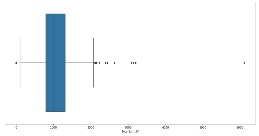
The boxplot chart gives us information about each feature's outliers.
	[{'cihi': 1018.5865615891045,
	'cilo': 967.4134384108955,
	'fliers': array([   0,    0,    0,    0,    0,    0,    0,    0,    0,    0,    0,
			0,    0,    0,    0,    0,    0,    0,    0,    0,    0,    0,
			0,    0,    0,    0,    0,    0,    0, 3094, 2110, 2136, 2633,
			2396, 6110, 2121, 2392, 3200, 2109, 3138, 3206, 2223, 2444, 2136,
			2153, 2158], dtype=int64),
	'iqr': 521.0,
	'mean': 1061.8043052837572,
	'med': 993.0,
	'q1': 793.0,
	'q3': 1314.0,
	'whishi': 2077,
	'whislo': 105}]
This information is used to cap the features' values
train_complet['TotalBsmtSF'] = train_complet['TotalBsmtSF'].clip(105,2077)
After having been capped, most of the features observe a rise in their correlation with the target feature. Indeed, for example, for the TotalBsmtSF feature, with a simple linear regression the R² score increases from 37,5% to 42%.


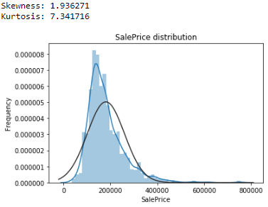
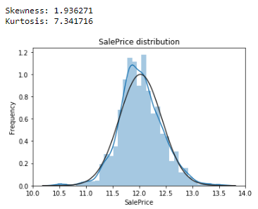
The target feature "SalePrice" has to be correctly distributed, the np.log1p() function offers the best correction. We can see here the effects of the np.log1p() function on the SalePrice feature distribution, before and after the transformation :
train["SalePrice"] = np.log1p(train["SalePrice"])
The continuous features can then be scaled. The methods used will be presented later.
	quantitative = ['LotFrontage','LotArea','YearBuilt','YearRemodAdd','MasVnrArea','BsmtFinSF1','BsmtFinSF2','BsmtUnfSF','TotalBsmtSF','1stFlrSF','2ndFlrSF','GrLivArea','GarageYrBlt','GarageArea','WoodDeckSF','OpenPorchSF','EnclosedPorch','ScreenPorch', 'GarageArea', 'GrLivArea', '1stFlrSF', 'TotalBsmtSF']
	for df in ['X_train','X_test','submission']:
		df = ownLibrary.scale_features_in_df(df, quantitative, scaleMethod)
The modified datasets are exported to csv. The following notebooks will now work on it without having to prepare again the data up to this waypoint.
	X_train['SalePrice'] = y_train
	X_train.to_csv ("path/Initial_train_rwrk.csv", index = False, header=True)
	X_test['SalePrice'] = y_test
	X_test.to_csv ("path/Initial_test_rwrk.csv", index = False, header=True)

	submission['SalePrice'] = 0
	submission.to_csv ("path/Initial_submission_rwrk.csv", index = False, header=True)
A hand-written function allows the testing of different combinations of feature transformation methods. Here we find the different scaling methods that can be applied to the dataset prepared earlier :
Another hand-written function allows the testing of different feature transformation methods :
The different results can then have their correlation with the target feature tested. A data frame give us the different scores and allows to chose the best method for each feature.
The two previously described functions produce a data frame containing the different R² scores. The following data frames are a shortened version of the complete one with fewer features and fewer scale methods concerned. The LotArea feature is an interesting one. The "natural" correlation (if no transformation at all) with the target feature SalePrice presents a R² of 8.54%. The data tree regressor manages to create bins that have a correlation of 20.20% which is a great improvement. The polynomial regression also improves the R² but not as much as the data tree regressor method. The second table indicates that these results can be improved again by scaling the feature before the transformations. The best results in the competition were obtained without feature scaling but with a large recourse to binning and polynomial regression.
Different transformations with non-scaled dataA parameter of the data tree regressor bins identifier function allow the printing of the bins as a python object. This object will later be used to replace the values of the different concerned features with another hand-written function.
	'LotFrontage': {
		1: [0,60.0],
		2: [61.0,74.0],
		3: [75.0,90.0],
		4: [91.0,220.0]
	},
	'LotArea': {
		1: [0,8635],
		2: [8640,10970],
		3: [10991,13680],
		4: [13682,430490]
	},
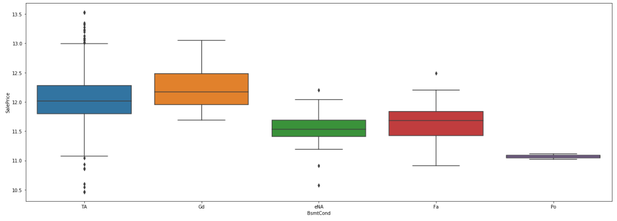
The method used to regroup categorical feature is based on a boxplot study. The boxplot show the correlation with the target feature for each state of a particular categorical feature. The similar states of this feature are then regrouped together. Here is an example with the BsmtCond feature. On the following picture, the correlation between each state of the feature and the target feature is represented with a boxplot. The blue boxplot and the brown won't be regrouped, because they aren't similar to any of the other boxplot. The last three states (eNa for no basement, Fa and Po) have more similar boxplots, so they will be regrouped together.
At the end of the study for each feature, another object python gives the list of states that will be regrouped later.
    'BsmtQual': {
        1: ["Ex"],
        2: ["Gd","TA"],
        3: ["Fa","eNA"]
    },
    'BsmtCond': {
        1: ["TA"],
        2: ["Gd"],
        3: ["Fa","Po","eNA"]
    },
Now that features have been analyzed and transformation methods chosen, the modeling part can start.
If the data preparation notebook hasn't done it, the continuous features are firstly scaled according to the method previously identified. Different lists of features are set for the rest of the process. Here, some continuous features are placed in lists for features which will be scaled (scaleMethod1 and 3) while some won't be scaled (scaleMethod0). We also retrieve the features which need a binning with the data tree regressor and those which need a polynomial transformation of order 2 or 3. The "ignore" list will be used by the dichotomization function.
Define the list of features for each transformation type
	scaleMethod0 = ['LotFrontage','YearBuilt','YearRemodAdd','GarageYrBlt','WoodDeckSF']
	scaleMethod1 = ['ScreenPorch','BsmtFinSF2','1stFlrSF','2ndFlrSF','TotalBsmtSF','GrLivArea']
	scaleMethod3 = ['EnclosedPorch','MasVnrArea','LotArea','BsmtUnfSF','OpenPorchSF','GarageArea','BsmtFinSF1']

	var_dtr = ['LotFrontage','YearBuilt','YearRemodAdd','GarageYrBlt','WoodDeckSF','BsmtFinSF2','LotArea','BsmtUnfSF','OpenPorchSF']
	var_base = ['Id', 'MiscVal', 'SalePrice', 'SalePrice_log']
	var_lr = ['ScreenPorch']
	var_base_pr2 = ['1stFlrSF','2ndFlrSF','GarageArea']
	var_base_pr3 = ['EnclosedPorch','MasVnrArea','TotalBsmtSF','GrLivArea','BsmtFinSF1']

	ignore = var_base + var_base_pr2 + var_base_pr3 + var_lr
The scaling function allows us to choose the method that will be used
	def scale_features(dataset, features, scaleMethod) :
	    from sklearn import preprocessing
	    if (features == [] or features == ''):
	        features = dataset.columns
	    df = copy.deepcopy(dataset)

	    if(scaleMethod == 0):
	        return df

	    if(scaleMethod == 1):
	        for var in df[features] :
	                df[var] = (df[var]-df[var].min()) / (df[var].max()-df[var].min())

	    if(scaleMethod == 2):
	        for var in df[features] :
	                df[var]=df[var]/df[var].max()

	    if(scaleMethod == 3):
	        for var in df[features] :
	                df[var] = (df[var]-df[var].mean()) / df[var].std()

	    if(scaleMethod == 4):
	        df = preprocessing.StandardScaler().fit(df[features]).transform(df[features])
	        df = pd.DataFrame(data=df[0:,0:],
	                      index=dataset.index,
	                      columns=dataset[features].columns)

	    return df
Performs the scale tranformation
	X_train = ownLibrary.scale_features(X_train, scaleMethod1, 1)
	X_test = ownLibrary.scale_features(X_test, scaleMethod1, 1)
	submission = ownLibrary.scale_features(submission, scaleMethod1, 1)
The states of categorical features are regrouped and the continuous features concerned are binned according to the data tree regressor bins. The regroupments are performed by a hand-written function. The function loops over a dataset's features. If a feature is in one of the python objects which define the regroupment, the regroupment is done.
Performs the regroupments and binning
    for column in dataset:
	    # ------------------------ If the feature is categorical ----------------------
	    if (column in ListeDesReglesQuali):
	        columnDiscretise = ownLibrary.discretise_1col_quali(dataset[column], column, ListeDesReglesQuali[column])
	        dataset.drop([column], axis=1, inplace=True)
	        dataset[column] = columnDiscretise

	    # ------------------------ If the feature is continuous ----------------------
	    elif (column in ListeDesReglesQuantiKB):
	        columnDiscretise = ownLibrary.discretise_1col_quanti(dataset[column], column, ListeDesReglesQuantiKB[column])
	        if( len(dataset[column]) != len(columnDiscretise)):
	            print('len(dataset[column]) != len(columnDiscretise) : ' + str(dataset[column]) + ' != ' + str(columnDiscretise))
	        else:
	            dataset.drop([column], axis=1, inplace=True)
	            dataset[column] = columnDiscretise
A group of new features can be created from the existing ones. For example, the number of fireplaces and their quality are combined to form one unique feature.
Creation of new features
	for df in [rgrpd_train, rgrpd_test, rgrpd_submission]:
		df["NewFirePlaces"] = df["Fireplaces"].astype(str) + df["FireplaceQu"].astype(str)
		df["NewExterQualCond"] = df["ExterQual"].astype(str) + df["ExterCond"].astype(str)
		df["NewCentrAirElec"] = df["CentralAir"].astype(str) + df["Electrical"].astype(str)
		df["NewKitchen"] = df["KitchenAbvGr"].astype(str) + df["KitchenQual"].astype(str)
		df["NewSale"] = df["SaleType"].astype(str) + df["SaleCondition"].astype(str)
A short hand-written function allows us to dichotomize a given dataset ignoring specified features. The ignored features are the continuous ones which haven't been binned, plus those which will undergo a polynomial transformation and a few others, such as the target feature.
The function that performs the dichotomization
    def dichotomize_dataset(dataset, columnsToNotDicho):
        dichotomizeDF = pd.DataFrame()
        for column in dataset :
            if(column not in columnsToNotDicho):
                dummies = pd.get_dummies(dataset[column], prefix=column)
                dummies.reset_index(drop=True, inplace=True)
                dichotomizeDF.reset_index(drop=True, inplace=True)
                dichotomizeDF = pd.concat([dichotomizeDF, dummies], axis=1, sort=True)
            else:
                dichotomizeDF[column] = dataset[column]
        return dichotomizeDF
Perform the dichotomization
	train_dicho = ownLibrary.dichotomize_dataset(rgrpd_train, ignore)
	test_dicho = ownLibrary.dichotomize_dataset(rgrpd_test, ignore)
	submission_dicho = ownLibrary.dichotomize_dataset(rgrpd_submission, ignore)
A hand-written function from the custom library performs a polynomial transformation on a list of features of a given dataset with a given polynomial order. The function returns the transformed dataset. Here a first polynomial transformation of order 2 on the concerned features is performed. The resulting dataset is then used for a second transformation of order 3 for another list of features defined at the begining of the notebook.
Perform the polynomial transformation
	train_pr2_transformed = ownLibrary.PolynomialRegrTransformationReturnDF(train_poly, var_base_pr2, 2)
	test_pr2_transformed = ownLibrary.PolynomialRegrTransformationReturnDF(test_poly, var_base_pr2, 2)
	submission_pr2_transformed = ownLibrary.PolynomialRegrTransformationReturnDF(submission_poly, var_base_pr2, 2)

	train_pr3_transformed = ownLibrary.PolynomialRegrTransformationReturnDF(train_pr2_transformed, var_base_pr3, 3)
	test_pr3_transformed = ownLibrary.PolynomialRegrTransformationReturnDF(test_pr2_transformed, var_base_pr3, 3)
	submission_pr3_transformed = ownLibrary.PolynomialRegrTransformationReturnDF(submission_pr2_transformed, var_base_pr3, 3)
At this stage, some datasets can have more features than others. For example, the lot area feature was transformed into several bins, but the train dataset has no bin number 1 of this feature. The harmonization inserts this feature/bin in the train dataset and fills it with 0 values (as the feature is a dichotomized one), indicating that no observations are concerned by this feature. Here is an example with the test dataset :
Identify the features which are present in the train and submission dataset but not in the test one
	a = train_rwrk.columns.difference(test_rwrk.columns)
	b = submission_rwrk.columns.difference(test_rwrk.columns)
	manqueTest = a.tolist() + b.tolist()
	print ('Result : ' + manqueTest)

	Result : ['Exterior1st_3', 'NewKitchen_23', 'Exterior1st_3', 'NewExterQualCond_12', 'NewKitchen_23']
Harmonization for the test dataset and result
	for colonne in manqueTest :
    	test_rwrk[colonne] = 0

	a = train_rwrk.columns.difference(test_rwrk.columns)
	b = submission_rwrk.columns.difference(test_rwrk.columns)
	manqueTest = a.tolist() + b.tolist()
	print ('Result : ' + manqueTest)

	Result : []
Several feature selection methods are used to detect effective combinations of features for the modeling part. The Stepwise provides a solution that presents a small set of features for a good accuracy. On the other hand, the Recursive feature addition maximizes the R² but uses more features.
A stepwise function found on the web leads to good accuracy modelings. The function has been included in the custom library and can be found at this address : Stepwise function's source The stepwise selection results in approximately 40 features, depending on the combination of scaling and transformation methods used. The R² score reaches around 90 %.
Perform a stepwise feature selection
	variables = list(train_rwrk.columns)
	ignore = ['SalePrice','Id','SalePrice_log']

	colonnes = [var for var in variables if var not in ignore ]

	X = pd.DataFrame(train_rwrk, columns=colonnes)
	y = train_rwrk['SalePrice_log']
	result_stepwise = ownLibrary.stepwise_selection(X, y)
The recursive feature addition is the most adapted to maximize the R² which reaches around 91,5 % of accuracy with around 90 features used. The function has been modified and included in the custom library from this post : Recursive feature addition function's source
The GridSearchCV library allows us to find the best parameters for a group of models. When these parameters are found, the features selected by the stepwise are transmitted to a hand-written function than runs several models fitted with the training data. The predicted values for each of these models are stored in two data frames, one for the training dataset predicted values, and one for the test dataset.
A last hand-written function prints the results of these modelings for the training and test datasets, giving information about overfitting or underfitting presence.
Define the features and models to use
	y = 'SalePrice_log'
	models = {
	    'fa' : {
	        'label' : 'Forêt aléatoire',
	        'function' : RandomForestRegressor(n_estimators=35, max_depth=11, min_samples_split=3, min_samples_leaf=1, random_state=0, n_jobs=-1)
	    },
	    ...
	    'mrl' : {
	        'label' : 'Regression linéaire multivariée',
	        'function' : LinearRegression()
	    }
	}
Perform the modeling
	for model in models :
	    models[model]['function'].fit(train_rwrk[var_stepwise], train_rwrk[y])
	predictions_train = ownLibrary.runModels1DS(train_rwrk, 'train', var_stepwise, y, models)
	predictions_test = ownLibrary.runModels1DS(test_rwrk, 'test', var_stepwise, y, models)
    ownLibrary.afficheResults(predictions_train, predictions_test, 'SalePrice', models)

    ---------- K-Nearest Neighbors ----------

        Train : R² = 61.2 %
        Test : R² = 56.2 %

    ---------- Decision Tree Regressor ----------

        Train : R² = 98.3 %
        Test : R² = 79.3 %

    ---------- Linear Regression ----------

        Train : R² = 91.5 %
        Test : R² = 91.7 %

    ---------- Random Forest ----------

        Train : R² = 97.5 %
        Test : R² = 85.7 %

    ---------- Ridge Regression ----------

        Train : R² = 91.4 %
        Test : R² = 91.5 %
The 91,7 % R² with the Multivariate linear regression is currently the best score obtained by the study. The submission on Kaggle.com ranks the study at 1,741, so in the first 33%.
Here is a summary of the steps that led to the result :

Feel free to access my Linkedin profile, have a look at my Github repository or send me a message via the contact page.